Expected Value of Conditional Probability Continuous
The three conditionals every data scientist should know
Conditional Expectation
Conditional expectation of a random variable is the value that we would expect it take, on the condition that another variable that it depends on, takes up a specific value.
If this sounds like a mouthful, despair not. We'll soon get to the 'a-ha' moment about this concept. To aid our quest, we'll use a Poisson distributed random variable Y as our protagonist.
So let Y be a Poisson distributed discrete random variable with mean rate of occurrence λ.
The Probability Mass Function of Y looks like the following. (PMF is just another name for the probability distribution of a discrete random variable):

The expected value of Y , denoted E ( Y ), is the sum of the product of:
- Every value of Y in its range [0, ∞], and,
- Its corresponding probability P( Y =y), picked off from its PMF. in other words, the following:

The thing with expected value is that if you were to put your money on any value of Y , E( Y ) is what you should bet on.
In case of Y which is Poisson(λ) distributed, it can be shown that E(Y) is simply λ. In sample distribution shown in the above graph, E( Y ) = 20.
If Y had been a continuous valued random variable such as a normally distributed random variable, E( Y ) is calculated as follows:

Where f(y) is the Probability Density Function (PDF) of Y and [a,b] is its range .
So what is conditional about this expectation? In this case, absolutely nothing, because Y , the way we have defined it, is an independent variable i.e. its value does not depend on any other variable's value.
We now introduce another protagonist: Variable X . With X in the picture, we can consider the situation where Y depends on X , i.e. Y is some function of X:
Y = f( X ).
A simple example of f(.) is a linear relationship between Y and X :
Y = β0 + β1*X
Where β0 is the intercept and β1 is the slope of the straight line.
Let's play God for a second. We'll claim to know the true relationship between Y and X. Let that relation be as follows (but don't let the regression modeler inside your head know this true relation!):
Y = 20 + 10 *X
Here is the plot of Y against X :

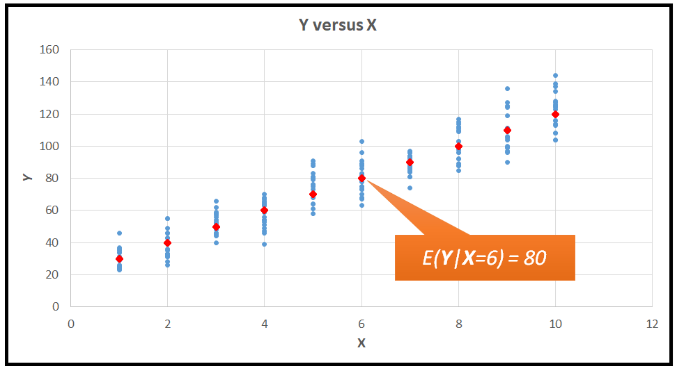
Wait, but isn't Y a random variable? Thus, for each value of X , we'd expect Y to take up one or more random values governed by probability distribution (PDF or PMF) of Y . And this sort of a random behavior of Y leads to the following kind of plot of Y versus X instead of the very neat plot we saw earlier:

Recollect once again that in our example, we have assumed that Y is Poisson(λ) distributed. It turns out that the parameter λ of the Poisson distribution's PMF forms the connective tissue between the neat straight-line plot of Y versus X we saw earlier and the smeared-over plot of Y versus X shown above. Specifically, λ is the following linear function of X :
λ( X ) = 20 + 10 *X
But as we noted at the beginning of the article, the expected value of a Poisson(λ) distributed random variable i.e. E( Y ), is simply λ. Therefore, it follows that for some value of X :
E( Y | X ) = λ( X ), and thus:
E( Y | X ) =20 + 10 *X
The notation E( Y | X ) is the conditional expectation of Y on X , or the expectation of Y conditioned on X taking a specific value 'x'.
For example, in the neat straight line plot of Y versus X, when X =6,
E( Y | X =6) = 20 + 10*6 = 80.
So now we can say that when X =6, Y is a Poisson distributed random variable with a mean value λ of 80.
We can carry out a similar calculation for every value of X to get the corresponding conditional expectation of Y on that value of X =x, in other words the corresponding mean λ for X =x. Doing so lets us 'superimpose' the two Y versus X plots as follows. The orange dots are the conditional mean values of the Poisson distributed sample of Y shown by the blue dots.
In general, if Y is a random variable having a linear relationship with X, we can represent this relation as follows:
E(Y|X =x ) = β0 + β1 * x
Where E(Y|X =x ) is called the Expectation of Y conditional upon X taking on the value x.
The conditional expectation, also known as the conditional mean of Y on X can also be written concisely as E( Y | X ).
Conditional Probability
We'll see how the explanatory variable X is about to 'work its way' into the Poisson distributed Y 's PMF via the parameter λ:
So far we have seen that:
E(Y|X =x ) = λ( X =x) = β0 + β1 * x
We also know that the PMF of Y is given by:

In the above equation, substitute λ with β0 + β1 * x, or indeed with any other function f( X ) of X , and bingo! The probability of Y taking up a particular value y is now suddenly dependent on X taking on a specific value x. See the updated PMF formula below:

In other words, the PMF of Y has now transformed into a conditional probability distribution function . Isn't that neat?
Y can have any sort of a probability distribution, discrete, continuous, or mixed. Similarly, Y can depend on X via any sort of a relation f(.) between Y and X . Thus, we can write the conditional expectation of Y on X as follows for the case when Y is a discrete random variable:
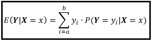
Where P( Y =y_i| X =x) is the conditional Probability Mass Function of Y .
If Y is a continuous random variable, we can write its conditional expectation as follows:

Where f( Y =y_i| X =x) is the conditional Probability Density Function of Y .
Conditional probability distributions and condition expectation occupy a prominent place in the specifications of regression models. We'll see the connection between the two in the context of linear regression.
Conditional Expectation and regression modeling
Suppose we are given a random sample of (y, x) tuples that are drawn from the population of values shown in the earlier plot:

Suppose also that you have decided to fit a linear regression model to this sample, with the goal of predicting Y from X. After your model is trained (i.e. fitted) to the sample, the model's regression equation can be specified as follows:
Y_(predicted) = β0_(fitted) + β1_(fitted)*X
Where β0_(fitted) and β1_(fitted) are the fitted model's coefficients. Let's skip through the fitting steps for now. The following plot shows how the fitted model looks like for the above sample plot. I've superimposed the conditional expectations of Y , E(Y|X) , for each value of X :

You can see from the plot that fitted model doesn't exactly pass through the conditional expectations of Y . It's off by a small amount in each case. Let's work out this error for X =8:
When X=8:
We know E(Y|X) because we are playing God and we know the exact equation between Y and X:
E(Y|X=8) = 20+10*8 = 100
Our model cannot know God's mind, so at best it can estimate E(Y|X):
Y_predicted|X=8 = 22.034 + 9.458 * 8 = 97.698
Thus the residual error ϵ for X=8 is 100 – 97.698 = 2.302
This way, we can find the residual errors for all other values of X also.
We can now use these residual error terms to express the conditional expectation of Y in terms of the fitted model's coefficients. This relationship for X =8 looks like this:
E( Y | X =8) =100 = 22.034 + 9.458 * 8 + 2.302
Or in general, we have:
E( Y | X ) = β0_(fitted) + β1_(fitted)*X + ϵ
in other words:
E(Y|X) = Y_(predicted) + ϵ
Where ϵ are the regression model's errors a.k.a. the residual errors of the model.
In general, for a 'well-behaved' model, as you train your model on larger and larger sample sizes, the following interesting things happen:
- The fitted model's coefficients, in our example: β0_(fitted) and β1_(fitted), start approaching the true values (in our example: 20 and 10 respectively).
- The fitted model's predictions ( Y_predicted ) start approaching the conditional expectation of Y on X , i.e. E( Y | X ).
- The model's residual errors start approaching zero.
Conditional Variance
Variance is a measure of the departure of your data from the mean.
Mathematically, the variance s² of a sample (or σ² of the population) is the sum of the squares of the differences between the sample (or population) values and the mean value of the sample (or population).

The following plot illustrates the concepts of unconditional variance s²( Y ) and the conditional variance s²( Y | X =x):

While the unconditional variance of the sample (or population) takes into account all the values in the sample (or population), the conditional variance focuses on only a subset of values of Y that correspond to the given value of X .
In our example, we define conditional variance of the sample s²( Y | X =x) as the variance of Y for a given value of X. Hence the notation s²( Y | X =x).
Conditional Variance and regression modeling
As with conditional expectation, conditional variance occupies a special place in the field of regression modeling, and that place is as follows:
The primary reason for building a regression model (or for that matter, any statistical model) is to try to 'explain' the variability in the dependent variable. One way to achieve this goal is by including relevant explanatory variables X in your model. The conditional variance gives you a way to explain by how much a regression variable has helped in reducing (i.e. explaining) the variance in Y .
If you find that the presence of an explanatory variable has not been able to explain much variance, it can be dropped from the model.
To illustrate this concept, let's once again look at the above plot showing the unconditional and conditional variance in Y.
The overall variance in the sample is 870.59. But if you were to fix X at 6, then just knowing that X is 6 has brought down the variance to only 25! The following table lists the conditional variance in Y for the remaining values of X. Compare each value to the overall, unconditional variance of Y, namely 870.59:

That's it! That's all there is to Conditional Probability, Condition Expectation and Condition Variance. You can see how useful and central a role these three concepts play in regression modeling.
Happy modeling!
Related
Getting to Know The Poisson Process And The Poisson Probability Distribution
PREVIOUS : Understanding Partial Auto-correlation And The PACF
NEXT : An In-depth Study of Conditional Variance and Conditional Covariance
UP: Table of Contents
Source: https://timeseriesreasoning.com/contents/conditionals/
0 Response to "Expected Value of Conditional Probability Continuous"
Post a Comment